Phase 1: Portfolio Construction & Overview
Baseline statistics for an 8-asset equal-weighted portfolio (SPY, QQQ, EFA, GLD, TLT, LQD, XOM, VNQ) over 2,514 trading days from 2015 to 2024. Diversification confirmed: portfolio volatility (11.7%) is below every individual asset. Excess kurtosis of 16.99 invalidates the normality assumption and motivates Historical Simulation and CVaR over parametric methods.
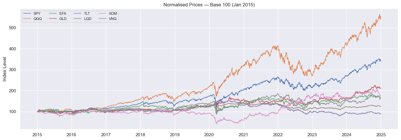
Normalised Cumulative Prices
All 8 assets rebased to 100. QQQ leads; TLT is the only negative total return. GLD and TLT show flight-to-safety during 2020.
Phase 1
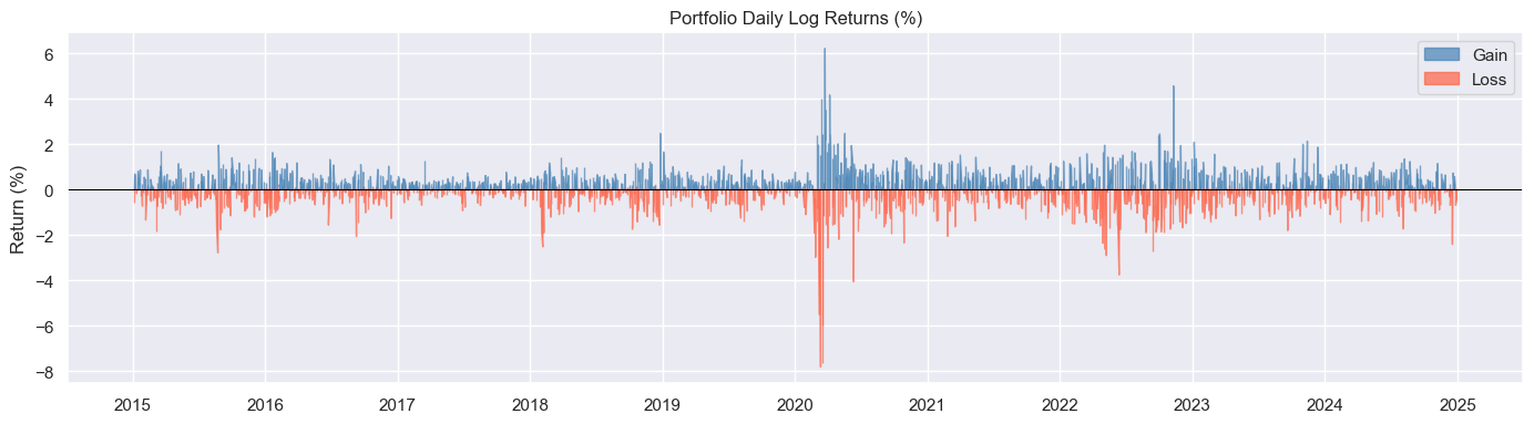
Daily Returns: Volatility Clustering
Calm stretches punctuated by violent bursts in 2020 and 2022. The pattern that motivates GARCH: bad days predict bad days.
Phase 1

Return Distribution vs Normal
Excess kurtosis = 16.99. The fat left tail is clearly visible against the Gaussian fit: the normality assumption is violated from the start.
Phase 1
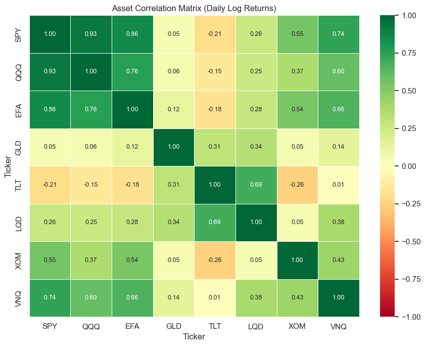
Asset Correlation Heatmap
TLT and GLD show low-to-negative correlation with equities. The 2022 rate shock broke this: both safety assets fell alongside equities.
Phase 1
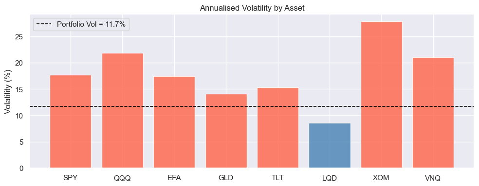
Asset Volatility Comparison
Portfolio vol (11.7%) sits below every individual asset. LQD lowest at 8.6%, XOM highest at 27.8%. Diversification confirmed.
Phase 1
Phase 2 & 3: VaR & CVaR / Expected Shortfall
Three VaR methods (Historical Simulation, Parametric, Monte Carlo) plus CVaR across 95% and 99% confidence levels. At 99%, Parametric VaR is lower than Historical Simulation: the normal distribution is too optimistic in the tail. CVaR/VaR ratio at 99% Historical = 1.68x vs the theoretical normal ratio of 1.16x: the empirical tail is 45% fatter than normality assumes. Basel III replaced VaR with CVaR for this exact reason.
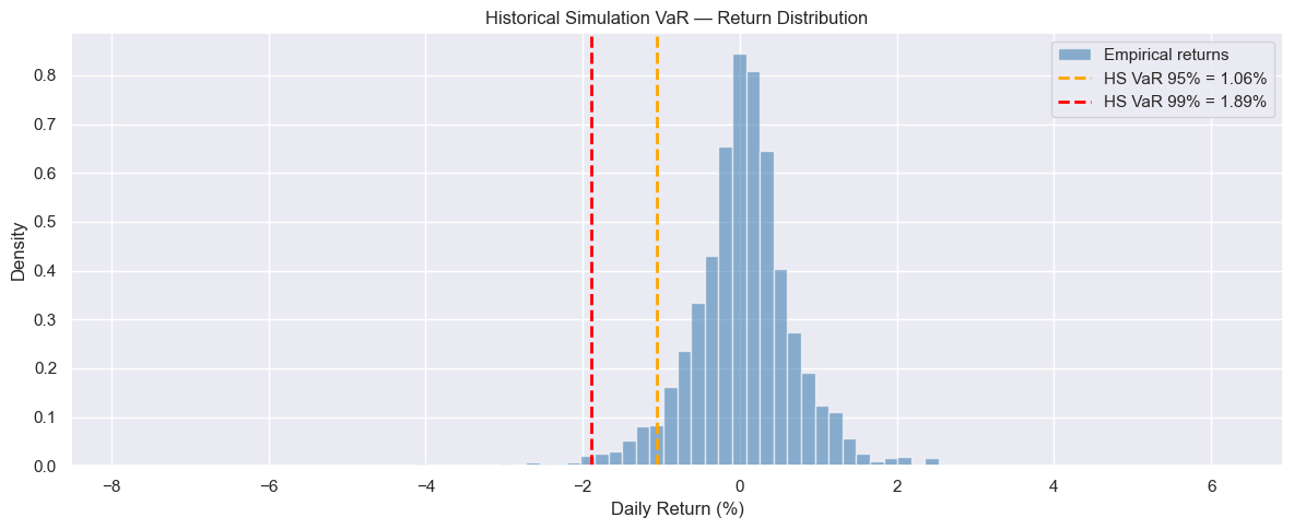
Historical Simulation: Return Distribution
Empirical left tail is thicker than normal. No distributional assumption: reads actual worst 1% of days. 99% VaR: $18,887.
Phase 2
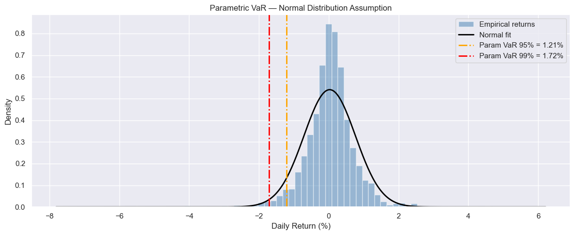
Parametric VaR: Normal Distribution Fit
Normal curve underestimates tail severity. 99% VaR: $17,159: $1,728 less than Historical Simulation. That gap is model risk.
Phase 2

Monte Carlo: 100,000 Simulated Paths
Converges to parametric result: simulation alone doesn't fix a wrong distributional assumption. 99% VaR: $17,007.
Phase 2
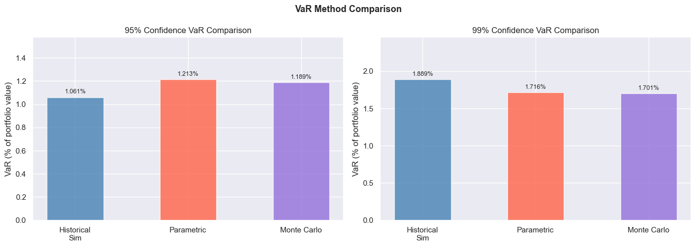
VaR Method Comparison
At 99%, HS exceeds Parametric: the ranking inverts from 95%. The inversion is the model risk gap that pre-2008 banks ignored.
Phase 2
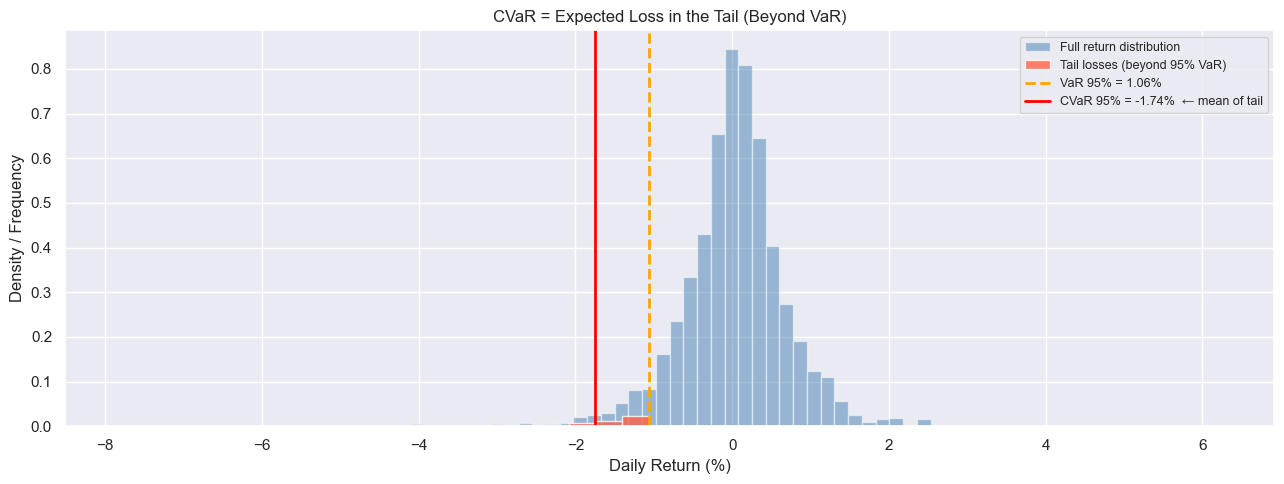
CVaR Tail Visualisation
CVaR = average loss beyond VaR. HS 99% CVaR: $31,791 vs VaR $18,887: ratio of 1.68x vs normal's 1.16x. Tail is 45% fatter.
Phase 3
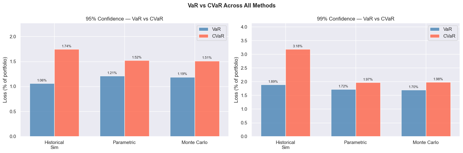
VaR vs CVaR: Bar Comparison
Historical CVaR exceeds Parametric and MC at both confidence levels. Gap widens at 99% where the normal assumption fails hardest.
Phase 3
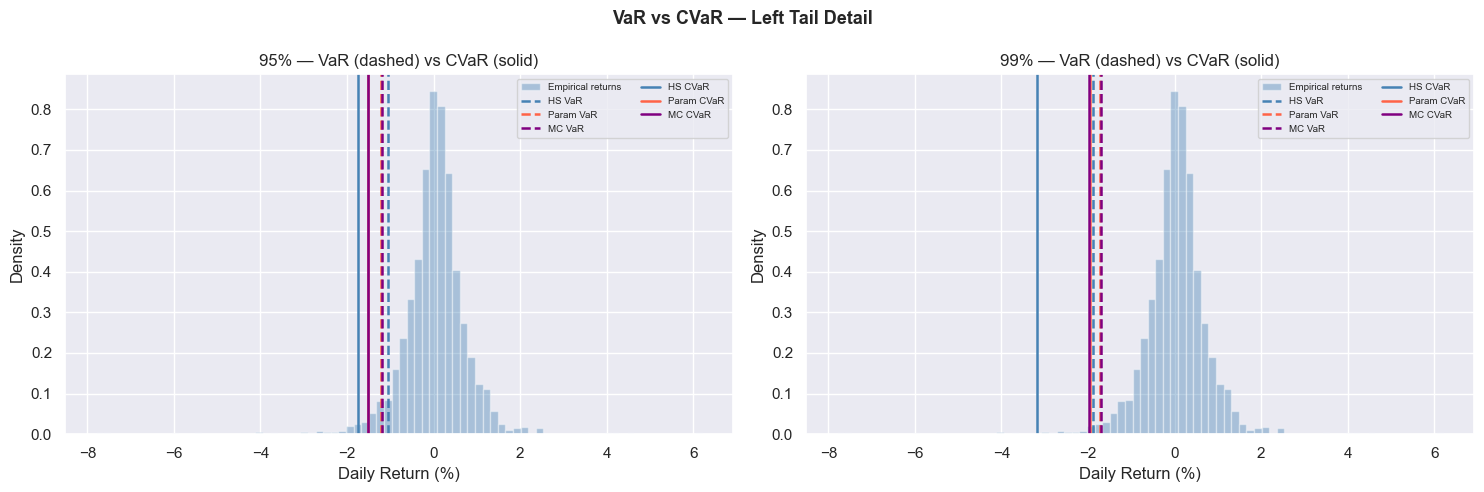
VaR vs CVaR: Distribution View
Meaningful probability mass sits beyond VaR in the empirical distribution. Normal models smooth this away.
Phase 3
Phase 4: Backtesting (Kupiec + Christoffersen)
Rolling 252-day out-of-sample VaR forecasts tested against actual returns using two statistical tests. Kupiec tests whether exception frequency is correct. Christoffersen tests whether exceptions cluster: a model passes only if breaches are random and independent. All three static models fail both tests at 99%. After one VaR breach, another the next day is 10x more likely (π11 = 14.3%). This failure motivates GARCH in Phase 7.
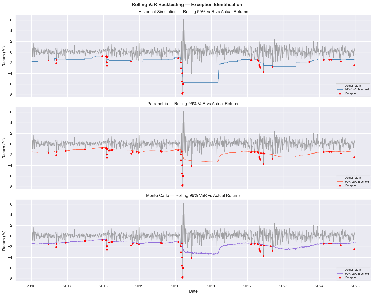
Rolling VaR vs Actual Returns
Static VaR barely widens during 2020. Breaches cluster precisely where the model should be widening: it has no memory of the regime shift.
Phase 4
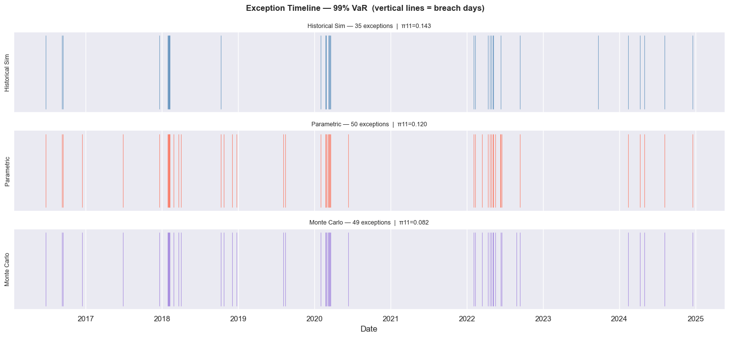
VaR Exception Timeline
Exceptions cluster visibly in 2020 and 2022. π11 = 14.3% for HS: after one breach, another the next day is 10x more likely than the unconditional rate.
Phase 4
Phase 5: Stress Testing
Historical crisis scenarios (GFC 2008–09, COVID 2020, Rate Shock 2022) and a hypothetical liquidity shock applied to the portfolio, benchmarked against VaR and CVaR. Every crisis scenario exceeds the 99% VaR threshold. COVID's worst single day was 4.14x the 99% VaR. The 2022 rate shock broke the negative stock-bond correlation assumed in the covariance matrix: both safety assets fell alongside equities.
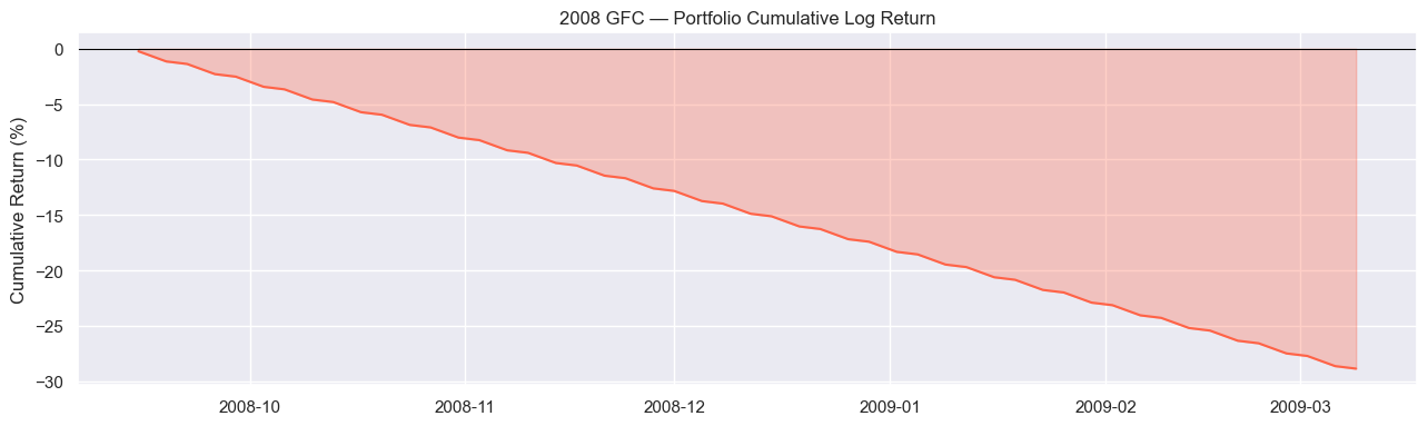
GFC 2008–09 Drawdown
28.9% total drawdown unfolding over months. Worst single day: 0.23%: the crisis built slowly but sustained for far longer than COVID.
Phase 5
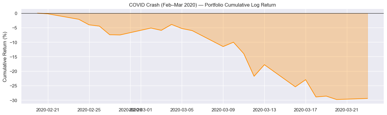
COVID Crash: Feb–Mar 2020
Worst single day: 7.81%: 4.14x the 99% VaR. Portfolio lost 29.5% peak-to-trough in weeks. Fastest crash in history.
Phase 5
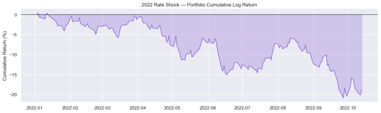
Rate Shock 2022
Both TLT and LQD fell alongside equities: the stock-bond negative correlation failed. Safety assets provided no protection at the worst moment.
Phase 5
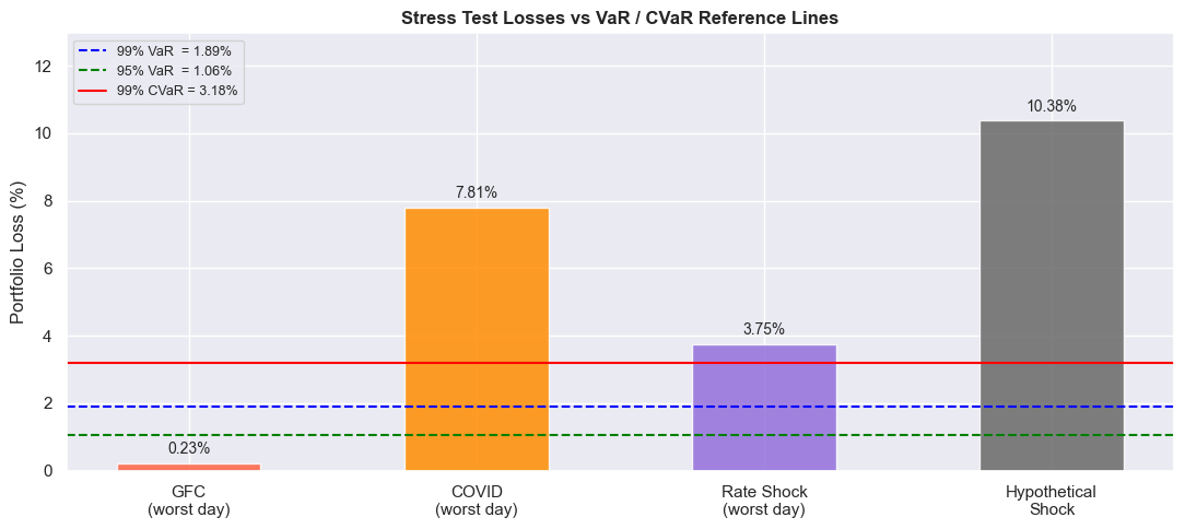
Stress Test vs VaR / CVaR Reference
All scenarios vs 99% VaR ($18,887) and CVaR ($31,791). Hypothetical shock: 5.49x VaR. COVID: 4.14x. Rate shock: 1.99x.
Phase 5
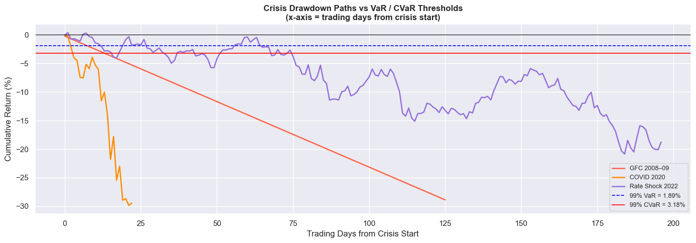
Crisis Paths Comparison
All crises overlaid. COVID and GFC both hit ~29% total loss via opposite trajectories: acute crash vs slow grind.
Phase 5
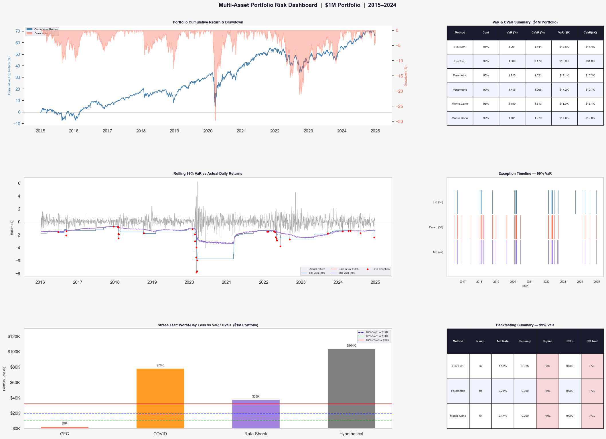
Risk Dashboard: Full Summary
Six-panel summary: cumulative return, drawdown, VaR/CVaR table, rolling backtest, exception timeline, stress test bar chart.
Phase 6
Phase 7: GARCH(1,1) with Student-t Innovations
Phase 4 showed all three static models fail both backtests at 99%. Root cause: static windows are blind to volatility regimes. GARCH(1,1) models time-varying conditional volatility: VaR thresholds automatically widen after large shocks. Pairing with Student-t innovations corrects the fat-tail underestimation. GARCH-t is the only model of five that passes both Kupiec and Christoffersen at 99%.
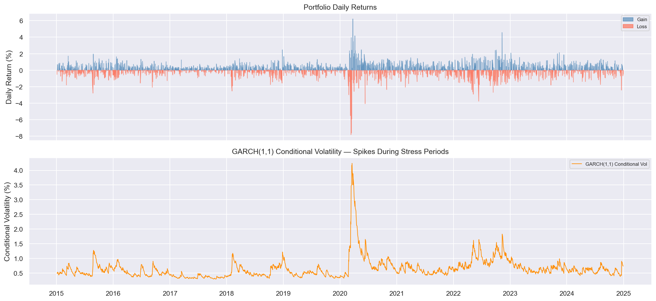
GARCH Conditional Volatility
Conditional vol spikes sharply in 2020 and 2022. Static windows average calm days into the estimate: GARCH reacts within one day.
Phase 7
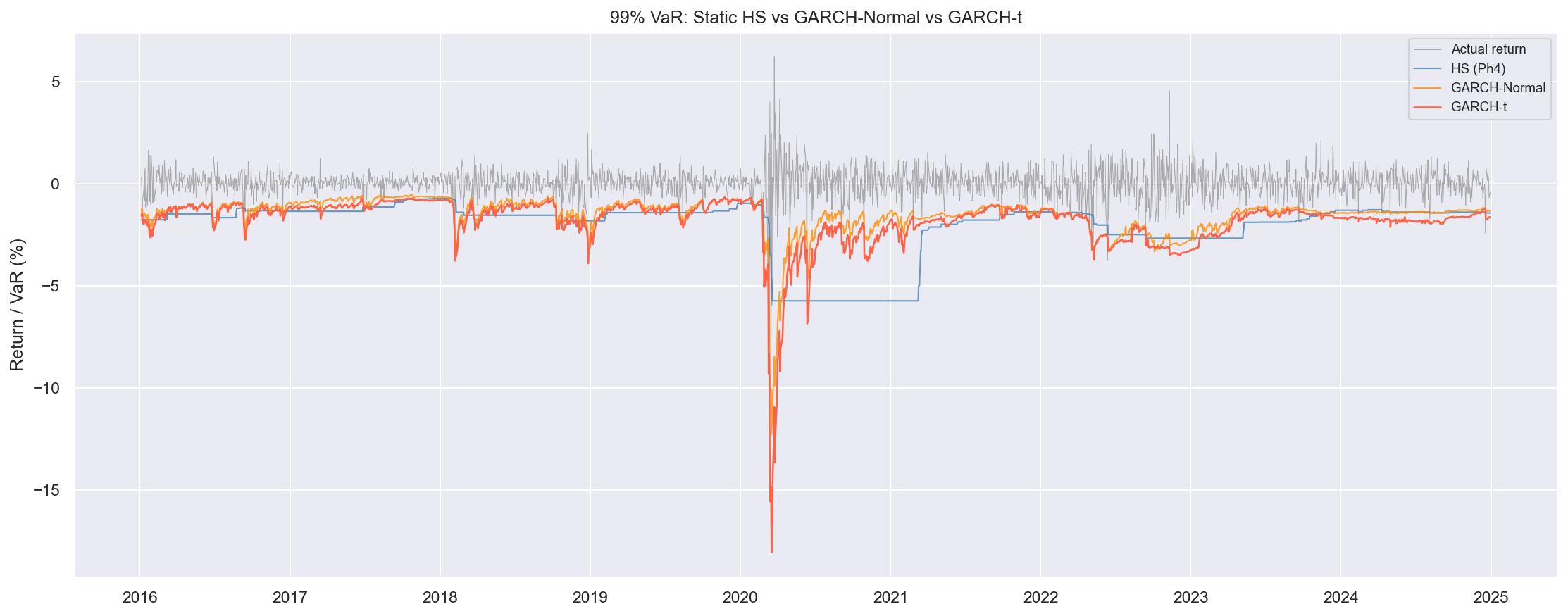
VaR Model Comparison: HS vs GARCH-Normal vs GARCH-t
GARCH-t (red) widens dramatically during stress. Static HS barely moves. The dynamic threshold is what allows GARCH-t to pass both regulatory tests.
Phase 7
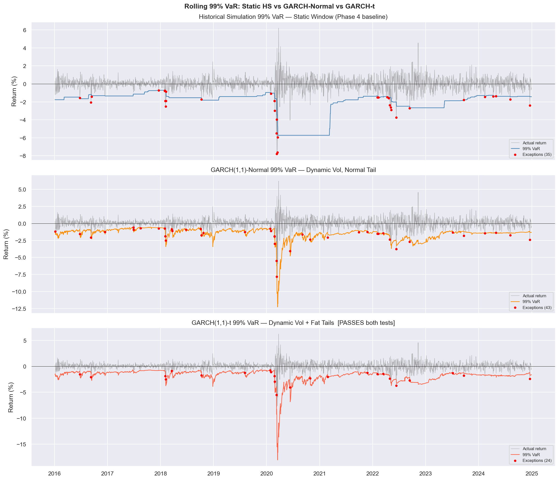
Exception Scatter: All Three Models
HS: 35 exceptions, clustered. GARCH-Normal: 43, less clustered. GARCH-t: 24 vs 22.6 expected, near-random: the only model that passes both tests.
Phase 7
Phase 8: Efficient Frontier & Portfolio Optimization
Phases 1–7 treated equal-weighting as given. Phase 8 solves the mean-variance optimization problem with long-only constraints across 60 target return levels to trace the efficient frontier, then extracts three portfolios: Minimum Variance, Maximum Sharpe (tangency), and Equal Weight (benchmark). The equal-weight portfolio sits inside the frontier: it is mean-variance inefficient. Portfolio construction choices directly affect tail risk, not just normal-times volatility.
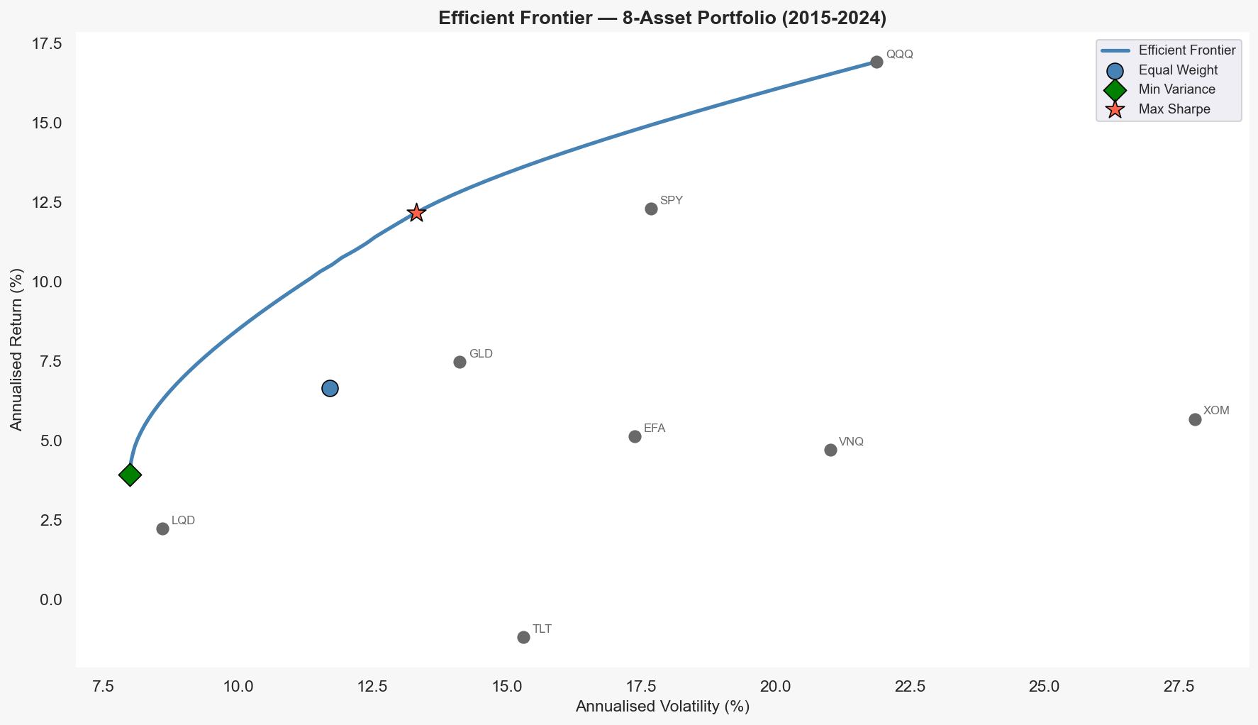
Efficient Frontier
Equal-weight portfolio sits inside the frontier: it is mean-variance inefficient. Both optimised portfolios dominate it on a risk-adjusted basis.
Phase 8
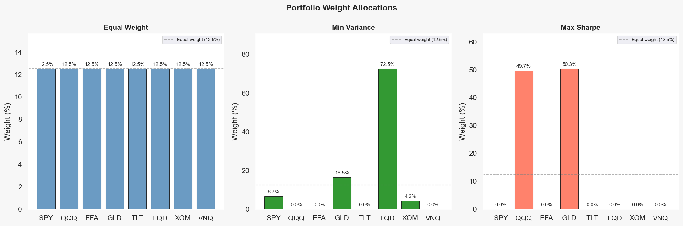
Optimised Portfolio Weights
Min Variance: concentrates in LQD, GLD, TLT. Max Sharpe: concentrates in QQQ, SPY. Equal weight: simple but dominated by both on risk-adjusted terms.
Phase 8